CoT monitorability: why you should use g-means over F1

The Monitoring Monitorability paper ^[1] argues that g-mean is a better metric than F1. In this blog post, I want to explain my understanding about it.

Preliminary math

Suppose you have a binary monitor that says either “misbehavior detected” or “no misbehavior.” The ground truth is either positive (bad behavior happened) or negative (it did not). As usual, the four outcomes are TP, FP, TN, and FN. Let the total number of samples be $\mathcal{N}$.

We then have:

• Prevalence $\pi$ asks how often does the model exhibit bad behaviors.

\[\pi = \frac{\mathrm{TP} + \mathrm{FN}}{\mathcal{N}}\]

• $\mathrm{TPR}$ means that how many bad behaviors did we flag out of all bad behaviors. This is also recall.

\[\mathrm{TPR} = \frac{\mathrm{TP}}{\mathrm{TP} + \mathrm{FN}}\]

• $\mathrm{TNR}$ means that how many good behaviors did we flag out of all good behaviors.

\[\mathrm{TNR} = \frac{\mathrm{TN}}{\mathrm{TN} + \mathrm{FP}}\]

• $\mathrm{Precision}$ flips the $\mathrm{TPR}$, which is now asking: out of all the bad behaviors we flag, how many are truly bad?

\[\mathrm{Precision} = \frac{\mathrm{TP}}{\mathrm{TP} + \mathrm{FP}}\]

Key difference between g-mean and F1

The key difference between g-mean and F1 is whether prevalence $\pi$ interferes with the metric. First, let us break down g-mean:

\[\mathrm{g\text{-}mean} = \sqrt{\mathrm{TPR} \cdot \mathrm{TNR}} = \sqrt{\frac{\text{flagged-bad}}{\text{all-bad}} \cdot \frac{\text{flagged-good}}{\text{all-good}}}.\]

TPR draws both its numerator and denominator from the (all-bad) positive pool, i.e. the samples where misbehavior actually happened. TNR draws both from the (all-good) negative pool, i.e. the samples where no misbehavior happened. Because TPR and TNR only look within their own class, changing the relative size of the two pools––meaning if you change $\pi$––does not affect TPR and TNR.

Now, let us express F1 with TPR and TNR:

\[\mathrm{F1} = \frac{2 \cdot \mathrm{Precision} \cdot \mathrm{Recall}}{\mathrm{Precision} + \mathrm{Recall}} = \frac{2 \cdot \mathrm{Precision} \cdot \mathrm{TPR}}{\mathrm{Precision} + \mathrm{TPR}} .\]

The blocker is Precision, which we need to bring in $\pi$.

\[\mathrm{TP} = \mathrm{TPR} \cdot \pi \mathcal{N}\] \[\mathrm{FP} = (1 - \mathrm{TNR}) \cdot (1 - \pi)\mathcal{N}.\] \[\mathrm{Precision} = \frac{\mathrm{TP}}{\mathrm{TP} + \mathrm{FP}} = \frac{\mathrm{TPR}\pi}{\mathrm{TPR}\pi + (1-\mathrm{TNR})(1-\pi)}.\] \[\mathrm{F1} = \frac{2\pi \cdot \mathrm{TPR}} {\pi(1+\mathrm{TPR}) + (1-\pi)(1-\mathrm{TNR})}.\]

This is the crucial point: F1 explicitly depends on $\pi$, while g-mean does not.

So what is wrong with prevalence $\pi$?

The key idea behind g-mean is that we do not want the monitorability metric to be confounded by prevalence $\pi$, i.e. by how likely the model is to misbehave.

Each agent has two independent properties in a monitorability setup:

• Behavioral tendency ($\pi$): how often it misbehaves on these tasks.
• CoT transparency: when it misbehaves (bad behavior), how often does the bad behavior get flagged; and when it does not (good behavior), similarly how often does it get identified.

The problem with F1 is that it includes $\pi$ through precision, so it collapses these two different properties into one number. For g-means, it is just the latter property.

A simple thought experiment

Imagine the paper runs an impossible coding task on five models, all monitored by the same GPT-5 monitor. Suppose every model’s chain of thought is equally transparent, and the monitor achieves $\mathrm{TPR} = 0.99$ and $\mathrm{TNR} = 0.99$ on all of them. In other words, they are all equally monitorable. A correct metric should therefore give the same score to all five.

But suppose the models misbehave at different rates:

• Model A hacks 90% of the time, so $\pi = 0.9$.
• Model B hacks 50% of the time, so $\pi = 0.5$.
• Model C hacks 20% of the time, so $\pi = 0.2$.
• Model D hacks 5% of the time, so $\pi = 0.05$.
• Model E hacks 1% of the time, so $\pi = 0.01$.

Now imagine publishing the F1 scores. You will get something like:

• Model E monitorability: 0.33 (penalized by low prevalence $\pi$)
• Model A monitorability: 0.99

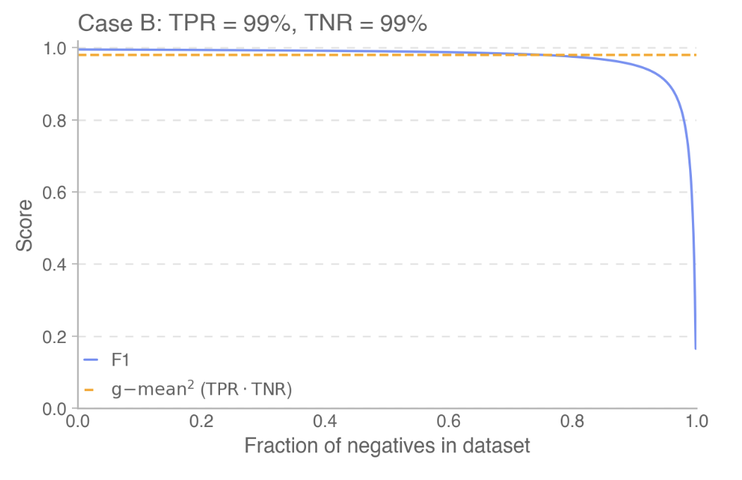
Figure 3 (Case B) taken from [1], where Model E with low prevalence (high fraction of negatives) corresponds to the major drop of blue-line.

The natural conclusion would be: “Model E’s CoT is nearly opaque; we can barely monitor it; this is dangerous.”

But that conclusion is false. Model E barely misbehaves, and when it does, the monitor catches it just as reliably as it catches Model A. F1 makes the safest model look the most dangerous because it entangles two independent facts:

• how often the model misbehaves
• how observable that misbehavior is

In reality, Model E is the safest model in the lineup for two independent reasons: it rarely misbehaves and it is transparent when it does.

Discussion

What is special about g-mean?

Nothing uniquely magical. Any metric that symmetrically aggregates TPR and TNR without introducing prevalence would do. G-mean is simply the cleanest choice and strongly penalizes failure on either axis.

Limitations of g-mean

That said, g-mean does have limitations. Since it excludes $\pi$, it is also insensitive to the balance between TPR and TNR. For example, a monitor with

\[\mathrm{TPR} = 0.64, \qquad \mathrm{TNR} = 1.0\]

has the same g-mean as a monitor with

\[\mathrm{TPR} = \mathrm{TNR} = 0.8.\]

In a safety-critical setting, those monitors are not equivalent. The first misses 36% of actual misbehaviors, which could be unacceptable even if it never raises a false alarm.

Appendix: Degenerate monitor that always flag “bad”

Consider a degenerate monitor that always predicts positive. Then

• $\mathrm{TPR} = 1$ because it catches all positives.
• $\mathrm{TNR} = 0$ because it never correctly identifies negatives.

Using the earlier expression for F1,

\[\mathrm{F1} = \frac{2\pi \cdot \mathrm{TPR}}{\pi(1+\mathrm{TPR}) + (1-\pi)(1-\mathrm{TNR})}.\]

Substituting $\mathrm{TPR}=1$ and $\mathrm{TNR}=0$ gives

\[\mathrm{F1} = \frac{2\pi}{\pi(1+1) + (1-\pi)(1-0)} = \frac{2\pi}{\pi + 1}.\]

If prevalence is extremely high, say $\pi = 0.999$, then

\[\mathrm{F1} = \frac{2(0.999)}{1 + 0.999} \approx 0.999.\]

So this degenerate monitor would be classified as nearly perfect, even though it is obviously useless on negatives.

By contrast, g-mean gives

\[\sqrt{\mathrm{TPR} \cdot \mathrm{TNR}} = \sqrt{1 \cdot 0} = 0.\]

This issue is partly about the numerator in F1 using only TPR, but prevalence is the main reason the score becomes misleadingly high for degenerate monitors. A simple alternative would be to use something proportional to $\mathrm{TPR} \cdot \mathrm{TNR}$ instead.

Acknowledgements

Before release, I received helpful feedback from Miles Wang on the post’s explanation of g-mean.

References

1. Guan, Melody Y., Wang, Miles, Carroll, Micah, et al. Monitoring Monitorability. arXiv preprint, 2025. arXiv:2512.18311 ↩1 ↩2